STARKs 101

A short walkthrough of how STARK proofs work

STARK 101

Ch1. Statement, LDE and Commitment

• Statement: There exists an x such that the 1023th ($a_{1022}$) value of the fibonacci square sequence is 2338775057. The whole sequence is under prime $P = 3221225473$

• As the prover we know that the value of x is 3141592. However this value should not be leaked to the STARK verifier.

• LDE (Low Degree Extension): Helps encode our sequence/data. Done in 3 steps:

  • Generate Input:

    • This is what our data looks like: $a_0, a_1, a_2,...., a_{1022}$

    • The above are the values of the first 1023 values in the fibonacci square sequence with the $a_0$ and $a_1$ set according to us (0 and 3141592)

    • This is also called the trace. Because this is like the trace of the computation.

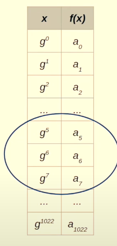
    • Now we choose another sequence of numbers, say $y_0, y_1, y_2,...., y_{1022}$

    • For our case we choose: $1, g^1, g^2, g^3,..., g^{1022}$ as the y-values for the trace values to be plotted on a graph

    • 

  • Interpolate Polynomial

    • Interpolate a polynomial such that for each $i$, $f(g^i) = a_i$

    • This is what it looks like:

    • 

  • Extend

    • Now, all you need to do is just evaluate the polynomial over a much larger domain as well.

    • In our case, it would be 8 times the original domain

    • In our case, the extended domain would look something like this: ${x_i'} = w, w.h, w.h^2,...., w.h^{8191}$

    • This is format of Reed-Solomon encoding/codeword.

    • Just as a reminder, this photo is for intuition only as this graph is drawn over a real field and has a smooth curve. In reality since this plotting is being done over a prime field, it would NOT look like this.

    • 

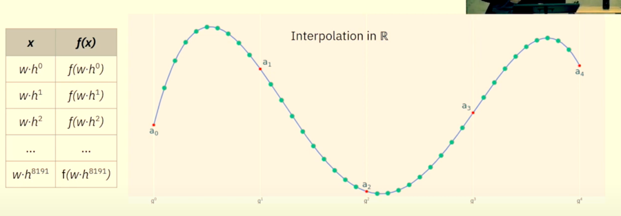
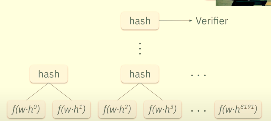
• Commitment: Now, we need to commit to our LDE.

  • To do this simply send the Merkle Tree root of the tree generated by hashing together all the values of the polynomial evaluation in the extended domain. That would look something like this:

  • 

Ch2. Polynomial Constraints

1. These are the few things that we will use in this chapter from the last chapter:

   • Trace - $a$
   • Generator of G - $g$
   • Trace Polynomial - $f(x)$

     • The polynomial formed by the interpolation of the trace values.

2. Constraints on ${a_n}$ that needs to be satisfied in order to convince the verifier of our statement

   • $a_0 = 1$
   • $a_{1022} = 2338775057$
   • $a_{n+2} = a_{n+1}^2 + a_n^2$
3. So the thing that we are going for is doing a bunch of reductions of these constraints so that we get another statement which if we prove to be true, then goes on to imply that these 3 initial constraints are also true.

2.1 Reduction 1

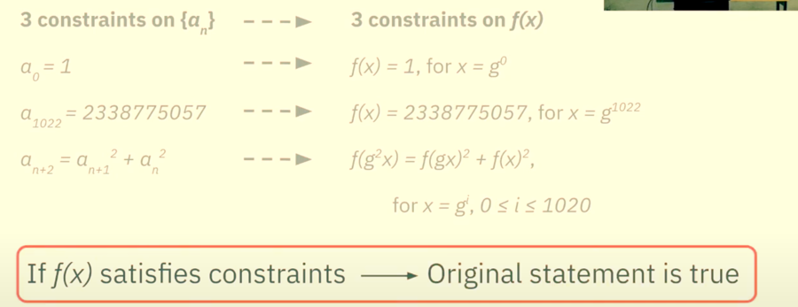
1. The first reduction is to convert the constraints on ${a_n}$ to constraints on the trace polynomial $f(x)$.
2. $a_0 = 1$ is the same as saying $f(x) = 1$, where $x$ is $g^0$.
3. Similarly, $a_{1022} = 2338775057$ can be thought of as $f(x) = 2338775057$ where $x = g^{1022}$
4. Lastly, the constraint $a_{n+2} = a_{n+1}^2 + a_n^2$ can be converted to:

   • $f(g^2x) = f(gx)^2 + f(x)^2$ for $x = g^i$, $0 \leq i \leq 1020$
5. This is all possible because of the way the trace polynomial was created. Just to jog thy memory, here's a photo:

   • 
6. Finally, at the end of Reduction 1, this is the state of affairs:

   • 

2.2 Reduction 2

1. So, instead of saying $f(x) = 1$ for $x = g^0$, we could also reframe that as:

   • $f(x) - 1 = 0$, for $x = g^0$
2. Similarly, $f(x) - 2338775057 = 0$, for $x = g^{1022}$
3. And lastly, $f(g^2x) - f(gx)^2 - f(x)^2 = 0$, for $x = g^i$, $0 \leq i \leq 1020$
4. So this basically means for the first constraint polynomial in this reduction, $g^0$ is a root
5. For the second constraint polynomial in this reduction, $g^{1022}$ is a root
6. For the last constraint polynomial in this reduction, $g^i$, $0 \leq i \leq 1020$ are the roots
7. Therefore, at the end of the second reduction this is the state of affairs:

   • 

2.3 Reduction 3

1. Given the theorem that if $(x-z)$ divides $p(x)$ then $z$ is a root of $p(x)$, the above reduction can be boiled down to the following:
2. $g^0$ is a root of $f(x) - 1$ can be written as:

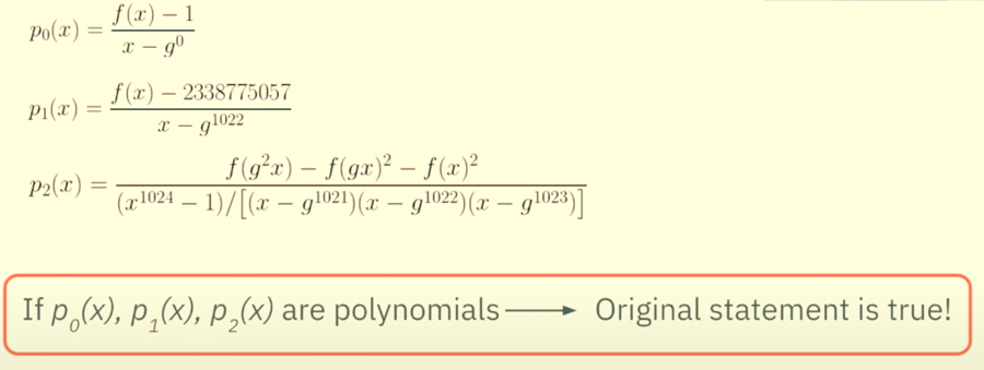
   • $(f(x) - 1) / (x - g^0)$ is a polynomial
3. $g^{1022}$ is a root of $f(x) - 2338775057$ can be written as:

   • $(f(x) - 2338775057) / (x - g^{1022})$ is a polynomial
4. And finally the last constraint can be re-written as:

   • $(f(g^2x) - f(gx)^2 - f(x)^2) / \prod_{i=0}^{1020}(x - g^i)$
5. Regarding point 4, the denominator is extremely inefficient and it has like 1021 roots and it's multiplication would be very hard for a computer. So, we do a couple of heavy optimizations.

6. $\prod_{i=0}^{1023}(x-g^i)$ can be written as $x^{1024} - 1$
7. ^^This polynomial is much easier to compute.

8. Now notice there is a difference in the $i$ values of pi. So to make it equivalent to $p_2x$ we divide the polynomial in 6 by the added $i$ value polynomials.
9. Then the final state of affairs after reduction 3 is the following:

   • 

A few more adjustments

1. Now we have established that we do not need to care about the initial constraints and all we need to do to prove our statement is to show that:

   • $p_0(x)$,$p_1(x)$,$p_2(x)$ are polynomials
2. 

   Screenshot 2024-11-23 at 4.06.51 PM
3. Now instead of showing 3 different rational functions to be polynomial, we can do the process once and for all.

4. Let's take a random linear combination of these three rational functions. That looks something like this:

   • $CP = \alpha_0.p_0(x) + \alpha_1.p_1(x) + \alpha_2.p_2(x)$
   • Where all the $\alpha$ are random field elements
   • We call it the composition polynomial

   • Luckily we have another theorem which states with very high probability that:

   • $CP$ is a polynomial $\iff$ all $p_i$'s are polynomials

Lastly

1. Commit to the CP using the Merkle Tree

Ch3. FRI Commitments

1. The goal here is to show that $CP$ is a polynomial which in turn will prove that all the constraints are satisfied and our initial statement was true.
2. And ofc, we won't prove what we want to prove.

   • We won't prove that $CP$ is a polynomial
   • We will prove that $CP$ is close to a polynomial of low degree.
3. Now, let us define what close and low degree mean.

4. Low degree is some agreement between the prover aand the verifier on some bounded degree that the polynomial is bounded by.

5. To understand Close, let us first understand distance.

   • The distance between function $f$ and polynomial $P$ is the number of points where $f(x) \neq p(x)$
   • For example, here the $f(x)$ and $p(x)$ disagree on 5 points, so the distance between them is 5.
   • 
   • So, a function $f$ is close to a polynomial $p$ if $D(f,p)$ is small.
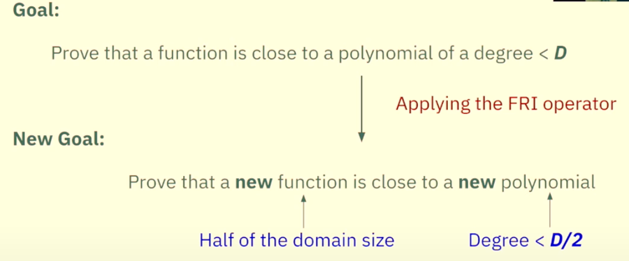
6. Our goal is to prove that the $CP$ is close to a polynomial of low degree. AND WE ACHIEVE THAT VIA FRI PROTOCOL.

   • FRI stands for Fast Reed-Solomon Interactive Oracles Proof of Proximity

3.1 FRI - The Protocol

• Receive random $\beta$
• Apply the FRI operator

• Commit (the resulting polynomial)

Repeat the above steps again and again until

• lastly the prover sends the result

  • at the stage where the degree has been reduced to the low degree agreed upon by the prover and verifier

• The FRI operator functions (broadly) on the following principle:

  • 

3.2 FRI Steps Overview

• 
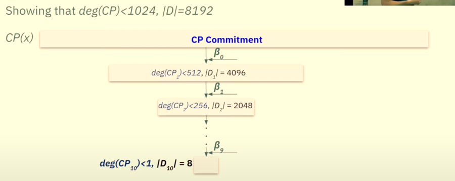
• As you can see above, $CP(x)$ keeps on getting halved until we have to prove $deg(CP_{10}) < 1$ and Domain is also less (8).
• The verifier stops sending random $\beta$ values now since a polynomial that is bounded by degree 1 is actually a constant.

3.3 Deep dive into the FRI operator

1. Each polynomial $P(x)$ can be split into an even and odd part like this:

   • $P(x) = g(x^2) + xh(x^2)$
2. Here's an example of the split $P_0(x) = 5x^5 + 3x^4 + 7x^3 + 2x^2 + x + 3$
3. It will be split into $g$ and $xh$ in the following fashion:

   • $g(x^2) = 3x^4 + 2x^2 + 3$
   • $xh(x^2) = 5x^5 + 7x^3 + x$
4. Now we receive the random $\beta$. This is what convinces the verifier that the prover didn't cheat, bc this can convince the verifier that the prover did not calculate the values in advance.
5. Now the new function will be:

   • $P_1(y) = g(y) + \beta h(y)$
   • Now $g(y) = 3y_2 + 2y + 3$
   • And $h(y) = 5y_2 + 7y + 1$
   • So, $P_1(y) = (3 + 5\beta)y^2 + (2 + 7\beta)y + 3 + \beta$
6. 

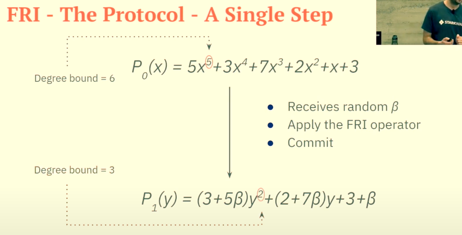
   Screenshot 2024-11-23 at 7.46.54 PM
7. As you can see in point 6, the bounded degree decreased from 6 to 3. We will keep on going like this until we reach an upper degree bound of 1.

8. Therefore, $deg(P_1) \leq deg(P_0)/2$

Ch4. The Proof

1. Up until now, we created a trace polynomial and commited to the trace root (Ch1)

2. Then we did some reductions on the original requirements on the trace and created the Composition Polynomial. We then committed to the CP root.

3. Then in Ch3 we applied the FRI protocol to prove that CP was close to a polynomial of a low-degree and we committed each layer of FRI, ie, $CP_1$ Root, $CP_2$ Root, ...., $CP_{10}$ Root.
4. This is what we have sent so far to the verifier from the prover's side. This is called the Commitment Phase.

5. The second part of the proof is called Decommitment or actually trying to convince the verifier that every calculation and commitment made so far was truthful and not false.

6. Now how this would work out is, that the verifier will send $q$ random elements and the prover will provide a validation data for each.
7. So, the first thing that needs to be proven by the prover to the verifier is the correct transition from trace polynomial to Composition Polynomial.

   • For that, the prover will send $f(x)$, $f(gx)$, $f(g^2x)$ for a given $x$.
   • This is enough information for the verifier to themselves calculate $CP_0(x)$, based on the formula below
   • 
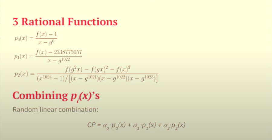
8. Now the next thing that needs to be proven to the verifier is the transition between each FRI layer. That is done via the following approach:

   • $CP_{i+1}(x^2) = g(x^2) + \beta h(x^2)$
   • And both $g(x^2)$ and $h(x^2)$ can be calculated only via $CP_i(x)$ and $CP_i(-x)$ like this:
   • 
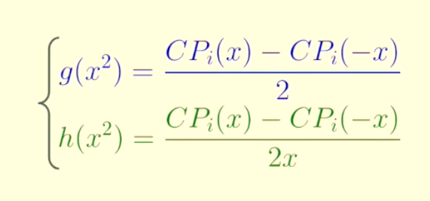
   • Therefore, the verifier can computer $CP_{i+1}(x^2)$ by only getting $CP_i(x)$ and $CP_i(-x)$ from the prover
9. Assuming that step 8 is clear, then the prover will send the value of $CP_1(-x^2)$ and from that value and from the $CP_1(x^2)$ calculated in step 8, the verifier will be able to check the value of $CP_2(x^4)$ and on and on until $CP_{10}$.
10. The prover is sending out these elements such as $f(x)$, $f(gx)$, $f(g^2)$, but remember we did not commit these individual elements but rather the hash of the merkle tree root, so how do we convince the verifier that we did indeed commit these elements into the Merkle tree?

    • So, the prover sends the verification path from the element to the Merkle tree to convince the verifier. This is called decommitment and looks something like this:

    • 
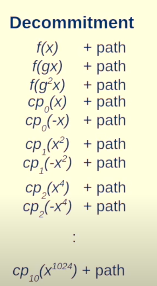
11. Now, the question is How Much data does the prover send to the verifier to convince him?

    • 
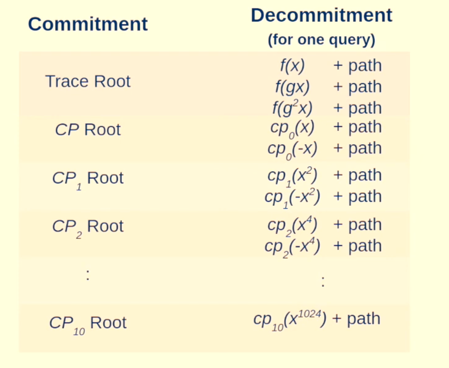
    • So, if you look at the left side (commitment), we are sending order of $log(n)$ elements in the commitment phase and then for a single query $q$, we are sending order of $log(n)$ path (from Merkle leaf to root). So, overall complexity is $O(log^2n)$
    • Now, for $q$ different queries, we need to send data in order of: $q * O(log^2n)$. But since $q$ is constant, the data remains of order $O(log^2n)$.

NOW AFTER ALL THIS SHENANIGANS, the VERIFIER IS CONVINCED THAT THE PROVER'S INITIAL STATEMENT ABOUT THE 1023rd VALUE OF THE SEQUENCE IS TRUE.